| Note: We strongly recommend to read the ICRA12 paper or chapter 4.2 in the PhD Thesis. |
| |
Introductory tutorial for using ethzasl_msf_sensor_fusion
Description: This tutorial is an introduction to Ethzasl MSF Framework. Using an offline data-set you learn how the framework works.Tutorial Level: INTERMEDIATE
Next Tutorial: custom_sensor_design
Contents
Overview and Preparation
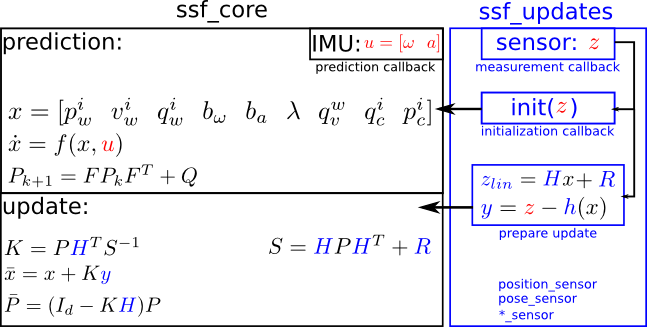
The Ethzasl MSF Framework stack is a multi-sensor fusion (msf) framework based on an Extended Kalman Filter (EKF). Multi sensor refers to one or more update sensors and the IMU as a fixed prediction sensor. The framework is essentially divided into the two EKF steps prediction and update. The prediction is made based on the system model (i.e. differential equations) and IMU readings. We do not take the IMU readings as update measurements since this would require matrix inversions and multiplications at IMU rate (which is in some cases up to 1kHz!).

In the above image, the red parts are sensor readings (from the IMU for prediction or from another sensor for the update). The blue parts are the parts which change if the update sensor type changes. The black parts are the constant (core) parts which stay analytically the same as long as we use an IMU for state propagation and the same state vector.
In the code, you will find:
p for pwi: the imu position in the world frame
v for vwi: the imu velocity in the world frame
q for qwi: the imu attitude in the world frame
b_w for bw: the gyro biases
b_a for ba: the accelerometer biases
L for λ: the visual scale factor with pmetric*λ = psensor
q_wv for q,,vw: the attitude between the update-sensor reference frame and the world reference frame
q_ci for qic: the attitude between IMU and the update-sensor
p_ci for pic: the distance between IMU and the update-sensor
As explained in this ICRA11 paper we use the error state representation in the EKF to facilitate computations with quaternions. An error quaternion is represented by δq=[1 θx θy θz]T where the 3-vector θ is used as state in the error state representation. This leads to a 25-states state-vetor.
From the software point of view, we wrap all constant (core) parts in the library msf_core. All parts that depend on the update sensor can then be added by the user via a module in msf_updates.
For this tutorial, you do not need any particular preparation other than downloading this dataset (3.7MB). It contains IMU data (linear accelerations and angular velocities) for the EKF prediction step. For the update step, it contains data from a 6DoF global pose-sensor (in this case, it is the position reading from a Vicon system).
Exploring the Dataset
In the dataset, we use for this tutorial, you find the following messages:
/auk/fcu/imu (type: sensor_msgs::Imu):
IMU readings of a micro helicopter (or a robot in general). It contains the 3D linear accelerations and 3D angular velocities at 100Hz./vicon/auk/auk (type: geometry_msgs::TransformStamped):
Vicon 6DoF pose readings. The data is recorded at 100Hz. The update-rate should not be equal or higher than the prediction rate.
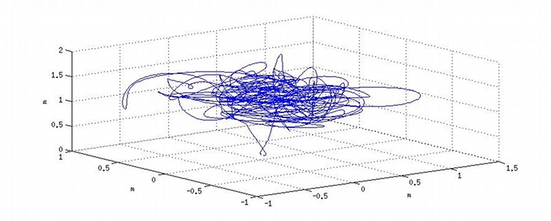
You may use rqt_plot to visualize the data and have a look in particular at the recorded pose in order to get an intuition of the movement of the robot in this dataset. Note: I actually was not able to do this with rqt_plot, but you should also try and make yourself comfortable with rviz to visualize data.

As you see, the 3D trajectory plot shows significant motion of the system. This motion is crucial in order to make the system states converge. This is proved in this paper. As a rule of thumb you should always excite at least two axes in acceleration and 2 axis in angular rates. A more detailed discussion on the excitation levels needed for state convergence can be found in this PhD Thesis, chapter 4.1.
NOTE: The system is in an unobservable mode if it is stationary. It needs a certain motion to make the states converge.
The General Setup
The core part of the framework (msg_core) is designed for the most general update sensor: an arbitrarily scaled 6DoF pose measurement with respect to its own reference frame which drifts in position and attitude with respect to a (gravity aligned) fix navigation frame. For example, such a sensor may be represented by using the 6DoF pose from a monocular visual odometry framework such as ethzasl_ptam.

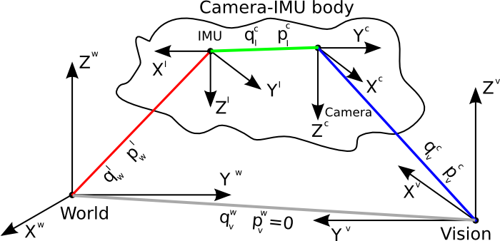
The above image depicts the frame setup of our framework: Each frame is connected with a certain translation p and rotation q (from quaternion) to another frame. The world frame is the frame in which our robot will navigate. The IMU and camera frame are centered in the respective sensors on the robot. The vision frame is the frame in which the visual part (e.g. ethzasl_ptam) triangulates the 3D features and with respect to which the visual part calculates the 6DoF camera pose. To represent the drifts occurring in every visual odometry framework (i.e. drift in visual scale, position and attitude) we introduce the so-called drift states in position pvw and attitude qvw.
The position drift is not observable since we do not have a global position measurement. Hence we do not use this state in this framework. The same is true for the attitude drift in yaw. This means that our "fix" world frame will drift in position and yaw together with the vision frame. However, roll and pitch drifts are observable and ensure that the world frame stays at least gravity aligned - a crucial property for MAV platforms. See a more detailed discussion on observability (also for multi-sensor systems) in this PhD Thesis.
Since the position drift is not observable we simply removed it in this framework. However, we are working with quaternions and the unobservable yaw cannot simply be set to zero by removing a state variable. Hence we introduce an artificial measurement keeping the yaw of the world frame aligned with the vision frame. Depending on the type of update sensor you use, additional such artificial measurements might be needed because other states might get unobservable.
For example, in this tutorial on the example of a 6DoF position update sensor, the attitude between IMU and the "camera" (i.e. the position sensor) is irrelevant and hence unobservable. Furthermore, assuming the Vicon frame is gravity aligned and not drifting, the attitude drift state between the "vision" frame (i.e. Vicon frame) and the world frame is superfluous as well. The same is true for the "visual" scale state, however, we keep this state in the state vector for a sanity check - it should converge to 1.
A Pose Sensor Example
Since the propagation step in this framework is always the same by using the IMU readings, we characterize the type of the multi-sensor-fusion framework by the sensor used for the filter update. In this example, we use a 6DoF global position sensor for the EKF update step. This can be a GPS sensor (3DoF), a Leica Totalstation or - in our case - the position readings from a Vicon system.
For every different update sensor, we need to incorporate the above mentioned steps (measurement callback, initialization and computation of H, y, and R) in a msg_updates module.
The msf_updates Module Files
Each update-sensor module consists of: Note: Not sure here. Need some help
In the directory /msf_updates/include/msf_updates/*_sensor_handler:
The file for the initialization routine *_measurements.h
the header and source file for the measurement callback and H, y, R computation *_sensorhandler.h and *_sensorhandler.hpp
In the directory /msf_updates/src/*_msf:
*_sensormanager.h
In the stack you already find pose, position, pressure and spherical sensor implementations, which represents a modules prepared for using a different DoF sensors as update sensor. In this example, we use a pose measurement from a Vicon system. Luckily in the new MSF framework, nearly everything is implemented.
Computing the Measurement Noise Matrix R
We assume that the Vicon has a fix covariance in its position measurement. Furthermore, the geometry_msgs::TransformStamped message contains no place for covariance information. Therefor we will set the position measurement noise fix later in the dynamic reconfigure gui.
A Note on the States in the System
As you remember, the system is originally designed to be used with a 6DoF arbitrarily scaled and drifting camera pose measurement. With this setup we require to consider states like
- 6DoF transformation between camera and IMU (translation and rotation)
- Visual scale (monocular system measure the position in arbitrary scale)
- Visual attitude drift with respect to a gravity aligned navigation frame
Depending on the sensor you use, not all these states are required - but they keep being in the core prediction model of the msf library. Hence, for states not used, we introduce artificial measurements to keep them bounded. Since they are not observable in the given sensor setup, this does not influence the estimate of the other states.
In the current example we can omit:
- rotation between the IMU and the sensor since we measure only absolute position
- visual attitude drift with respect to a gravity aligned navigation frame. We are sure that the Vicon measurements do not drift. Furthermore, in this tutorial, the Vicon frame is gravity aligned.
In this example we keep the "visual" scale in the state vector as sanity check of the filter performance - of course this state should converge to 1 when using Vicon position measurements.
Because of the above reasons, the measurement noise matrix R has 6 fix entries of 1e-6 (3 for the rotation between sensor and IMU, 3 for the visual attitude drift) to reflect low noise on the artificial measurements.
Computing the Measurement Matrix H and the Residuals y
We leave this part to the next tutorial.
For this tutorial, no changes in the computation of the measurement matrix H and the residuals y are necessary since the original code is already made for a 6DoF position sensor. In the code, note the artificial measurements for the unobservable states mentioned above.
Compiling the MSF Viconpos Sensor Framework
In order to run the framework, you need a main file that creates a class of the above new designed update-sensor module. Watch that you already have a main.cpp in /src/pose_msf.
In CMakeLists.txt we have already defined the new module as well.
Try and compile the framework correctly. If you cannot compile the framework because you are getting error with glog or catkin, clone asctec_mav_framework, catkin-simple and glog_catkin.
The framework must be compiled within a catkin workspace (how to create a catkin workspace):
$catkin_init_workspace
$catkin_make
$source devel/setup.bash
Running the MSF Viconpos Sensor Framework
Once the framework compiles all the original repo, we have to make a couple of changes to test it with the dataset provided above.
Getting the new Namespace
$roslaunch viconpos_sensor.launch
You should see a line that reads: “Loading parameters for pose sensor from namespace: /msf_viconpos_sensor/pose_sensor You will have to replace the first part of your viconpos_sensor_fix.yaml references to that namespace. ISSUE to be fixed in the original repo here. If not I have learnt that the parameters of the fix file don't ever get loaded.
Modifying the parameter (.fix) file
- In msf_updates/viconpos_sensor_fix.yaml, replace all the /pose_sensor/pose_sensor/ with /msf_viconpos_sensor/pose_sensor/ (Or whatever you have on your namespace. Do NOT replace the ones that have msf_core.
- In msf_updates/viconpos_sensor_fix.yaml, change the data_playback parameter to true because we are going to be playing data from a rosbag and check that the fixed_covariance parameter is also set to true (which should already be).
Remaping topics and launching the filter automatically
Inside /msf_updates/launch/viconpos_sensor.launch, add these two lines before the <rosparam> line:
<remap from="/msf_core/imu_state_input" to="/auk/fcu/imu"  />
<remap from="msf_updates/transform_input" to="/vicon/auk/auk" />
You are here basically remaping filter input topics to the topics that the rosbag will be publishing. You are not changing any outputs of the system, but only listening to different input topics for the same message and data.
- To initialize the filter we have two ways. You can run in a new terminal:
$rosrun rqt_reconfigure rqt_reconfigure, then go to the pose_sensor and click on the init_filter button. Or, you can create a ros service call in the launch file to do this for you. To do this, just add this line AFTER your node in the viconpos_sensor.launch.
<node pkg="rosservice" type="rosservice" name="initialize" args="call --wait /msf_viconpos_sensor/pose_sensor/initialize_msf_scale 1"/>
Launching the Framework
roslaunch msf_updates viconpos_sensor.launch
This should launch the viconpos_sensor framework. If your filter was initialized correctly, or if you are going to do rosin qt_reconfigure rat_reconfigure, then after you do that, you should see:
[ WARN] [[some time stamp]]: No measurements received yet to initialize attitude - using [1 0 0 0]
[ INFO] [[some time stamp]]: filter initialized to:
position: [some value, some value, some value]
scale:1
attitude (w,x,y,z): [1, -0, -0, -0]
p_ci: [0, 0, 0]
q_ci: (w,x,y,z): [1, 0, 0, 0]
The warning is OK since we have not yet sent any attitude data to the system. This warning could be removed in the initialization routine in viconpos_measurements.h.
Then run the data playback in pause mode and from t=25s on - before the MAV was standing still and thus was in an unobservable mode.
rosbag play dataset.bag --pause -s 25
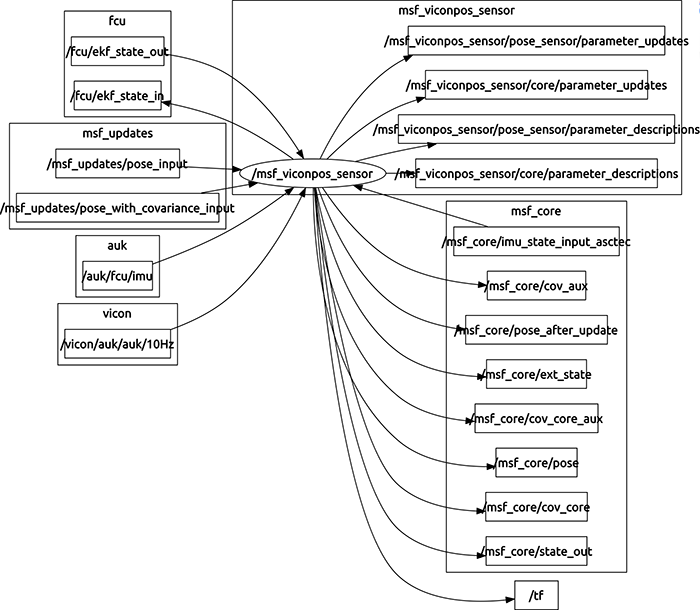
The framework is now ready. Before you hit play for the playback, read further to learn how to visualize the data. A rqt_graph should look like the following

Visualizing the Data
We provide a couple of scripts to visualize the different states of the filter. But since they are still written with the old rxplot command, we must update them:
Go to msf_core/scripts/plot_relevant Change rxplot for rqt_plot and delete everything starting at –b. Leave only the first rqt_plot command as it will not open several windows as rxplot did. Just leave the parameters you want to look at. I recommend starting with:
rqt_plot msf_core/state_out/data[0]:data[1]:data[2] # Positions
Which will give you (x,y,z) filtered position of the quad.
For a quick sanity check you may call
rosrun msf_core plot_relevant
Now you can start the data replay and observe the behavior of the filter. You may notice that the visual scale factor is very sensitive to correct initialization and prone to get stuck in local minima.
Note that the plot scripts use the /msf_core/state_out message. This message appears with an update measurement and contains the full state vector. You may also plot other messages:
* /msf_core/pose: is a PoseWithCovarianceStamped published at prediction (i.e. IMU) rate and containing the 6DoF IMU pose w.r.t. the world frame. You may use this message for vehicle control.
* /msf_core/ext_state: this is a legacy message to be used with the Luenberger observer with an AscTec platform. We discuss this in the asctec_hl_interface tutorial. It contains the 6DoF IMU pose and the 3DoF velocity without any covariance entries and is published at IMU rate
* /msf_core/correction: contains the correction vector to be applied to the current state before the update. This is to be used with an AscTec platform discussed in sFly tutorial. It is published at update-sensor rate.
Extra Important Notes
Please note that the frequency of the Vicon data is here divided by 5. This means that you are actually only getting 20Hz out of the Vicon and 100Hz out of the IMU, so it's expected if you get very tiny small jumps every now and then.


